Point Cloud Tangles

This page is a read-only extract from an interactive tangle software tutorial, with the same title, which is offered in the form of a jupyter notebook on our GitHub page. The steps required to run it are described there, in the 'getting started' section.

To follow the tutorial, you should first read the following chapters of Diestel's Tangles book.

• Chapter 1.3, Tangles in data science;
• Chapter 6.1, Indirect clustering by separation: hard, soft or fuzzy;
• Chapter 7.4, The evolution of tangles: hierarchies and order;
• (if you're ambitious) Chapters 14.1 and$~$14.2.

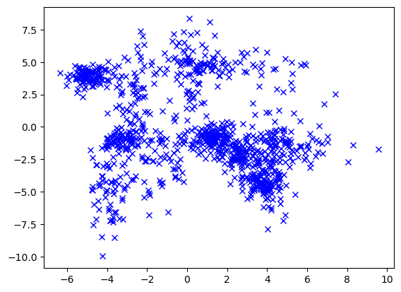
We will use Tangles to find soft clusters in point clouds in the plane:

Potential features in generic clustering such as this are partitions of the dataset into two subsets; features, therefore, are subsets of the set of all data points, those appearing as one side of one of those partitions.

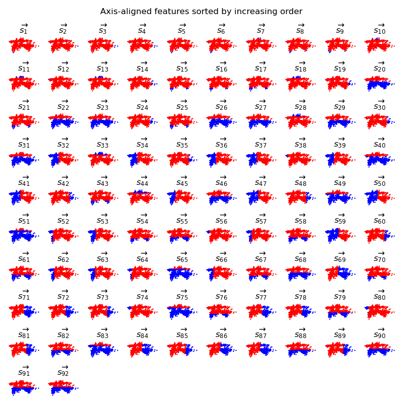
To demonstrate the power of tangles, we use a deliberately simple feature system, one obtained without even looking at the dataset: we simply use $50$ horizontal and $50$ vertical lines, equally spaced, which each partition the entire set of data points into two subsets.

We then use an order function from Chapter$~9.1$ of the Tangles book to separate the wheat from the chaff: we compute tangles first of those potential features, or partitions, that have low order. Those are the partitions that divide few pairs of close data points. These partitions are no more sophisticated than before, though: they are still given by a single horizontal or vertical dividing line.

Our 100 partitions are shown in the table below (after removing duplicates), in increasing order. Horizontal and vertical partitions are not considered separately.

Note that the partitions of lowest order, those at the top of the table, are not the most useful: they have low order simply because they separate only few data points from all the others, and split 'few close pairs' only for that reason. But as we allow the order of our partitions to increase, some of the partitions are more balanced.

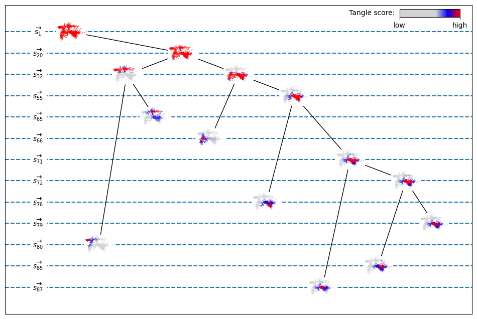
Specifying our partitions in increasing order, we can now build a tangle search tree (Chapter$~11.2$):

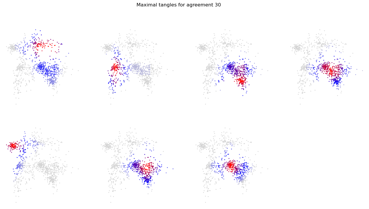
For each of the 14 tangles shown, a heat map shows how much each data point agrees with that tangle: the bright-red points are those which, for many of the partitions oriented by that tangle, lie on the side to which the tangle orients that partition. We call the number of those partitions the score of that point for the given tangle. Data points are shown red in the tangles for which they score highly, blue for tangles for which they score less highly, and grey for tangles that orient most partitions away from that point.

Note that tangles that orient more partitions, those further down in the diagram, are more focussed: only few points are shown red in those tangles, as it points to a smaller area or denser cluster. The seven lowest tangles in the diagram, the leaves of the tangle search tree, are shown again more clearly below: