Tangles in Images II

This page is a read-only extract from an interactive tangle software tutorial, with the same title, which is offered in the form of a jupyter notebook on our GitHub page. The steps required to run it are described there, in the 'getting started' section.

In this tutorial we search for tangles in Leonardo's Mona Lisa. The notebook is inspired by the first of all tangle application papers, Tangles and the Mona Lisa. This has now been superseded by the following chapters of the Tangles book:

• Chapter 6.2, Tangles of pixels: clusters in images;
• Chapter 14.6, Image segmentation, identification, compression.

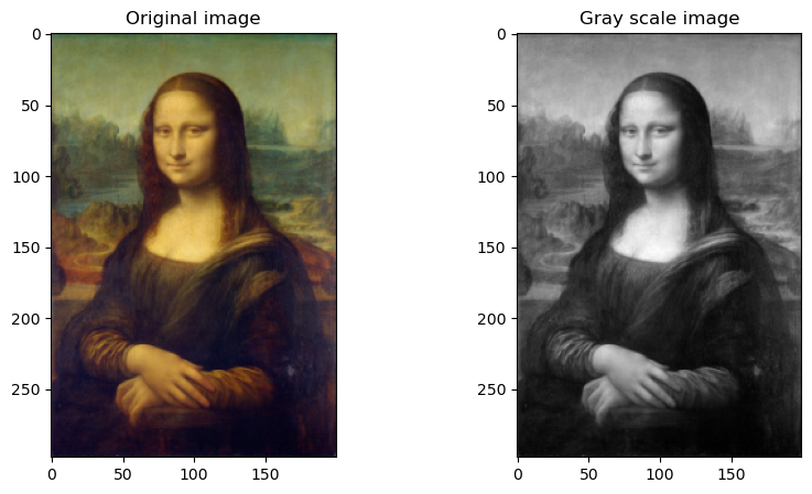
Let's have a look at the painting. For simplicity, we will work here with the gray scale image.

In image analysis, potential features are partitions of the set of pixels into two subsets, so features are subsets of the set of pixels. In this tangle application we use spectral features, as defined in Chapter$~10.2$ of the book.

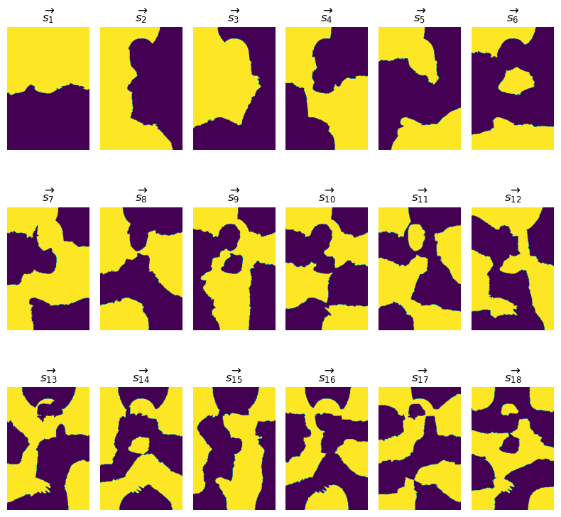
To find these spectral features, the eigenvectors for a certain matrix are computed, and for every eigenvector a feature corresponding to its positive entries is created. The simplest features found in this way are shown below in yellow, in increasing order of their corresponding eigenvalues:

We see that the degree of fragmentation of these features increases with their corresponding eigenvalues: features for small eigenvalues are simpler than those for larger eigenvalues.

There is no single feature which, by itself, detects any local structures or recognizable segment in the picture. But this is not a problem for tangles: rather, it is their forte to find structure in the combination of even the simplest features if there are enough of those.

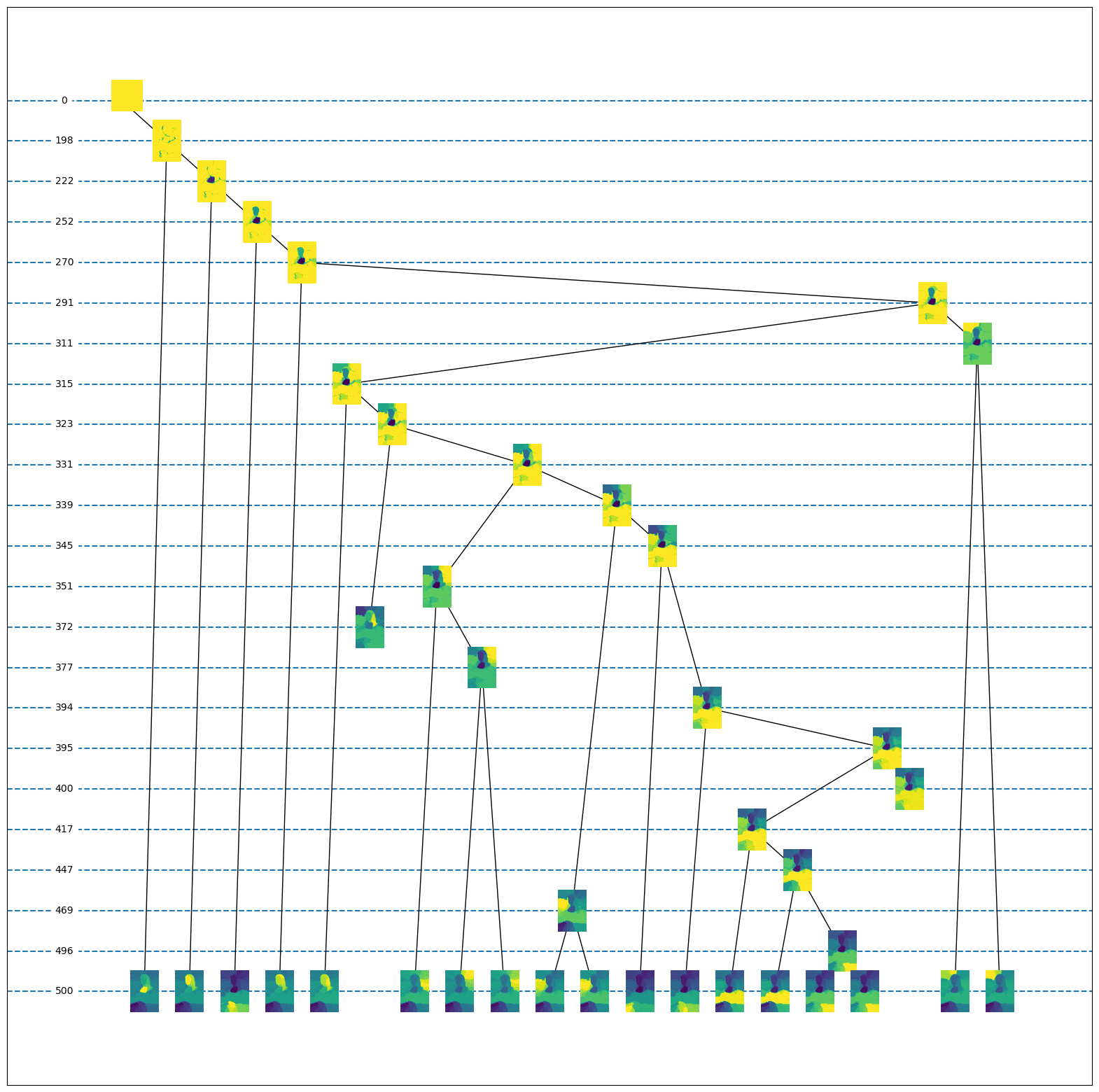
The next plot shows a portion of the tangle search tree (Chapter$~11.2$), and visualisations of the tangles at different levels of this tree. Every tangle is drawn as a heat map, where the intensity of each pixel indicates how much it 'belongs' to that tangle. More formally, a point is bright in the image for a tangle if for many of the partitions it lies on the side chosen by that tangle. Tangles further down in the diagram specify more of the potential features than those higher up, and therefore show more detail:

We can see how the tangles split into more refined tangles as they specify more and more potential features: those corresponding to our 18 eigenvectors, but also some corners of these features (Chapter$~7.4$). One of these tangles dies prematurely at level$~377$; compare 'fake tangles' in Chapter$~11.2$. We are particularly interested in the tangles that are leaves of the tangle search tree: those that specify all our potential features.

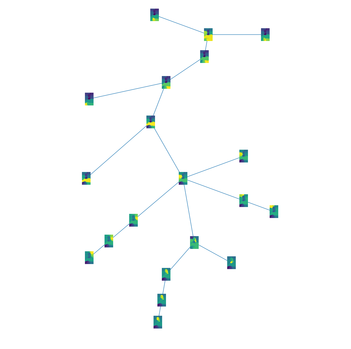
Finally, we computed the tree of tangles as in Chapter$~11.3$. This is shown below. It allows us to visualize our tangles in a tree structure and thereby gives an overview of how they are related.

The tangles in the lower branch of the tree, for example, zoom in on Mona Lisa's face and segment it into its constituent parts.